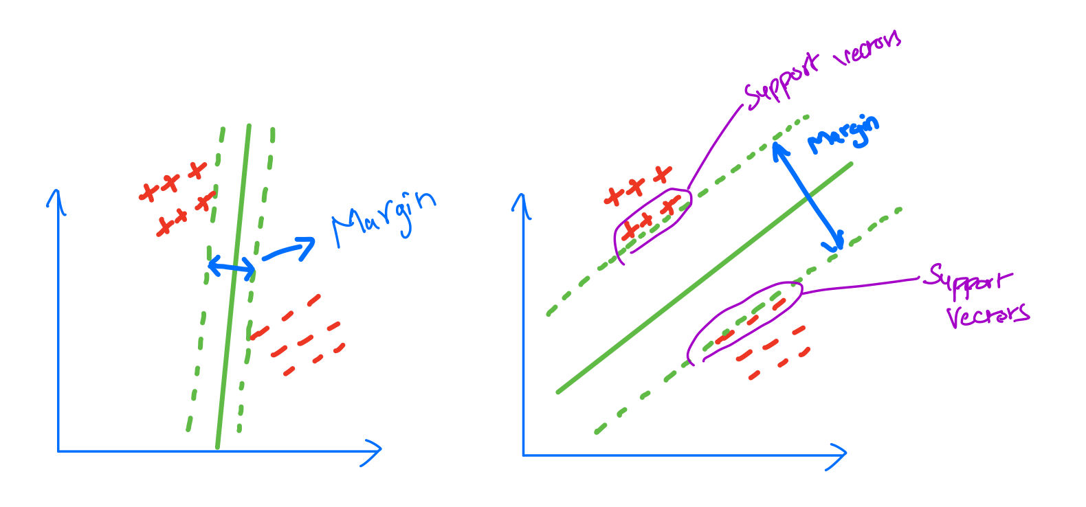
SVM aims to make the margings as large as possible between closest data points of those classes.

Key ideas

• find hyperplane that separates the class
• increase the margin that separates the class
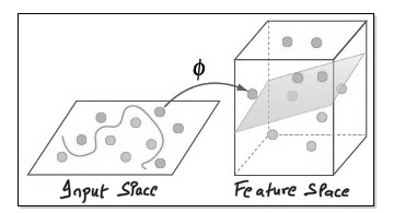
• use kernal spec to make the model work for Non Linear data.

Applications

• Handwriting recognition
• facial recognition

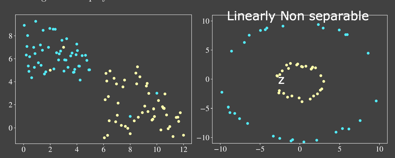
we can apply it for Linear as well as Non Linear. For Non Linear data we will use kerner spec.

Linear vs Non Linear

Usecases

• regression
• classification

Hypothesis function

Lets say we have training samples ${(x_i, y_i), i=1 to n}$ where $x_i \in {R}$ are input training samples and $y_i$ where $y_i \in {-1, +1}$ are class attributes i.e output classifications.

Lets assume these are linearly separable, then there exist vector $w \in R$ and scalar $b \in R$

$w^T x_i + b > 0, \forall i \text{ such that } y_i = +1$

$w^T x_i + b < 0, \forall i \text{ such that } y_i = -1$

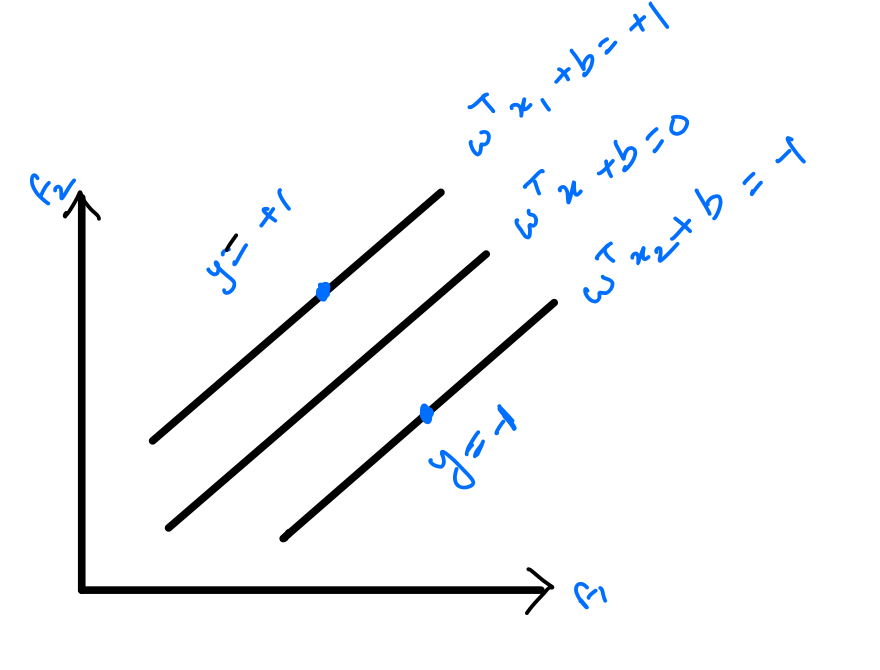
Since the classes are linearly separable, there exists a line that separates the 2 classes.

$w_T x + b = 0$

By scaling above equation, we can also find such that there will be no samples existing between these hyperplanes.

$w_T x + b \geq 1, \forall i \text{ such that } y_i = +1$ $w_T x + b \leq -1, \forall i \text{ such that } y_i = -1$

The above equations can also be written as….

$y_i * [w^T x_i + b ] \geq 1, i \in {1…n}$

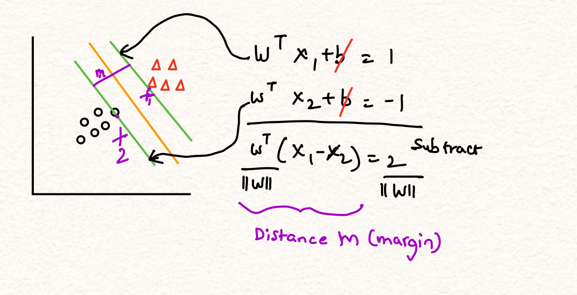
The distance between these equations is called margin

Goal of SVM

To find the max margin between the hyperplanes such that there will be no data points in between them.

SVM margin width

Optimization problem

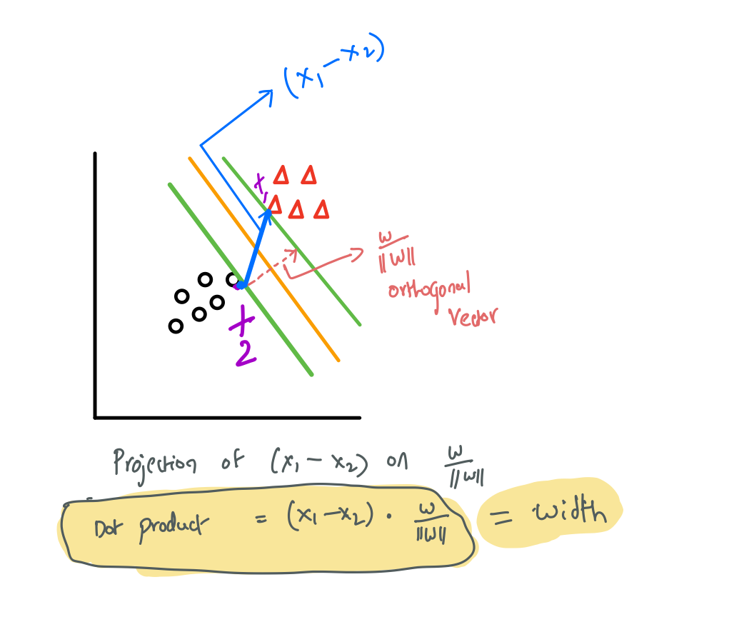
The width equation $\frac{2}{||w||}$ also can be taken as $\frac{1}{2* ||w||^2}$ which is $\frac{1}{2 * w^T * w}$

Maximize $\frac{2}{||w||}$ mean minimize $\frac{1}{2 * w^T * w}$

For Hard Margin SVM

Minimize : $\Phi(\mathbf{w})=1 / 2 \mathbf{w}^{T} \mathbf{w}$

Subject to $: y_{i}\left(\mathbf{w}^{T} \mathbf{x}_{\mathbf{i}}+b\right)-1 \geq 0 \quad \forall i$

Integrating constraints into lagrangian form…

Note: Minimize $: J(\mathbf{w}, b, \boldsymbol{\alpha})=1 / 2 \mathbf{w}^{T} \mathbf{w}-\sum_{i=1}^{N} \alpha_{i} y_{i}\left(\mathbf{w}^{T} \mathbf{x}{\mathbf{i}}+b\right)+\sum{i=1}^{N} \alpha_{i}$

Note: Subject to $: \alpha_{i} \geq 0 \quad \forall i$

Minimize J wrt $w$ and $b$ and maximize wrt $\alpha$

SVM Types

using kernel spec

# load iris dataset

from matplotlib import pyplot as plt
from sklearn import datasets
from sklearn.model_selection import train_test_split
import pandas as pd
import seaborn as sns

iris = datasets.load_iris()

iris_df = pd.DataFrame(iris.data, columns=iris.feature_names)
iris_df['target'] = iris.target
iris_df = iris_df.loc[iris_df['target'].isin([0,1])]
iris_df.head()

.dataframe tbody tr th {
    vertical-align: top;
}

.dataframe thead th {
    text-align: right;
}

iris_df.shape

(100, 5)

# visualize
sns.lmplot(x='petal length (cm)',y='petal width (cm)',hue='target',data=iris_df, fit_reg=False)
plt.xlabel('petal length (scaled)', fontsize = 18)
plt.ylabel('petal width (scaled)', fontsize = 18)
plt.show()

# separate input and output variables from dataframe
X=iris_df.iloc[0:3]
y=iris.iloc[:,4]

X_train, X_test, y_train, y_test = train_test_split(iris.data, iris.target, test_size=0.33, random_state=42)

# train the model with default hyperparameter
from sklearn.svm import SVC
from sklearn import metrics
svc=SVC() #Default hyperparameters
svc.fit(X_train,y_train)
y_pred=svc.predict(X_test)
print('Accuracy Score:')
print(metrics.accuracy_score(y_test,y_pred))

Accuracy Score:
1.0

# print confusion matrix 
print(metrics.confusion_matrix(y_test, y_pred))

[[19  0  0]
 [ 0 15  0]
 [ 0  0 16]]